By Gautam Sathu, Andras Miczak, Dorothy Marshall,
Rob Campbell
Simulation
Any analytical method meant
to imitate a real-life system, especially when other analyses are too
mathematically complex or too difficult to reproduce is called a simulation.
Without the aid of simulation, a spreadsheet model will only reveal a single
outcome, generally the most likely or average scenario. Spreadsheet risk
analysis uses both a spreadsheet model and simulation to automatically analyze
the effect of varying inputs on outputs of the modeled system.
Monte Carlo
Simulation
Monte Carlo
Simulation is a standard technique for simulating real-world situations
involving elements of uncertainty. Monte
Carlo is used extensively in finance for such tasks as pricing derivatives or
estimating the value at risk of a portfolio.
Software
Crystal Ball 2000 Standard is an easy-to-use simulation program that helps you analyzes the risks and uncertainties associated with your Microsoft Excel spreadsheet models. As a fully integrated Excel add-in program with its own toolbar and menus, Crystal Ball picks up where spreadsheets end by letting you perform Monte Carlo analysis. Crystal Ball automates the cumbersome "what-if" process using Monte Carlo simulation, by applying a range of values or a probability distribution to each uncertain variable. The program generates random values from within the defined probability ranges, and then recalculates the model literally hundreds or thousands of times, storing the results of each "what-if" scenario. This timesaving process alleviates having to manually enter different scenarios over and over again
Why use MCS for
complex situations?
A simulation
calculates multiple scenarios of a model by repeatedly sampling values from the
probability distributions for the uncertain variables and using those values
for the cell. Crystal Ball 2000 simulations can consist of as many trials (or
scenarios) as you want - hundreds or even thousands - in just a few seconds.
During a single trial,
Crystal Ball randomly selects a value from the defined possibilities (the range
and shape of the distribution) for each uncertain variable and then
recalculates the spreadsheet.
What do you do with uncertain variables in your spreadsheet?
For
each uncertain variable (one that has a range of possible values), you define
the possible values with a probability distribution. The type of distribution
you select is based on the conditions surrounding that variable. Distribution
types include:


 and
and  .
.
To add this sort of
function to an Excel spreadsheet, you would need to know the equation that
represents this distribution. With Crystal Ball 2000, these equations are
automatically calculated for you. Crystal Ball 2000 can even fit a distribution
to any historical data that you might have.
Monte Carlo Simulation: Application
Based on the data we had for
our previous project, we determined the two external variables (variables
beyond the company’s control) as Average Price and Average Advertising. Our
decision variables, Price and Advertising are variables that have to be chosen
by the company’s Manager. The output variable Firm Demand is what the Manager
is interested in. In making his decision, the Manager will first use historical
data to get statistical information on the external variables. This will help
him specify the minimum and maximum values while specifying values for his
simulation model. The mean also gives him an idea about the most likely value.
After having obtained this
information, the Manager goes ahead and defines the assumptions associated with
each external variable and chooses the type of distribution that is most
appropriate. In our case, we chose a triangular distribution for the Average
price, and a Normal distribution for the Average advertising. For the normal
distribution, we obtain the standard deviation from the statistical analysis,
and input this value along with the mean.
At this point, the company’s
Manager needs to decide what values he wants for his decision variables. Based
on historical data, we decided to have our Price = $385 and our Advertising
expense to be $98000.
We go ahead and choose the
output variable, which is Firm Demand, and then run the simulation for 1000
trials. A bar chart is generated with the probable outcomes and the number of
units that must be produced for that probability to exist. These values are a
good indicator of whether the company is right in its estimated value of the
decision variables.
Data Set
|
Quarter |
Avg_Price |
Avg_Adv |
TID |
|
1 |
387.5 |
77000 |
12020 |
|
2 |
382.9 |
84870 |
14820 |
|
3 |
378.1 |
91860 |
18140 |
|
4 |
384.1 |
78510 |
16610 |
|
5 |
378.5 |
93400 |
18400 |
|
6 |
380.6 |
90550 |
19580 |
|
7 |
378.9 |
100410 |
22270 |
|
8 |
383 |
99820 |
21740 |
|
9 |
383.2 |
83600 |
16380 |
|
10 |
379.4 |
90860 |
17390 |
|
11 |
372 |
104660 |
25800 |
|
12 |
367.2 |
108570 |
28390 |
|
13 |
378.3 |
88420 |
16430 |
|
14 |
382 |
76800 |
15960 |
|
15 |
379 |
101240 |
23060 |
|
16 |
377 |
103750 |
24410 |
|
17 |
372.7 |
98200 |
23580 |
|
18 |
368.5 |
96670 |
25050 |
|
19 |
365 |
104000 |
32850 |
|
Average price summary statistics |
|
Average Advertising Summary Statistics |
||
|
|
|
|
|
|
|
Mean |
377.8 |
|
Mean |
93325.8 |
|
Standard Error |
1.4 |
|
Standard Error |
2254.7 |
|
Median |
378.9 |
|
Median |
93400.0 |
|
Mode |
#N/A |
|
Mode |
#N/A |
|
Standard
Deviation |
6.1 |
|
Standard
Deviation |
9828.0 |
|
Sample Variance |
37.2 |
|
Sample Variance |
96590470.2 |
|
Kurtosis |
-0.1 |
|
Kurtosis |
-1.0 |
|
Skewness |
-0.7 |
|
Skewness |
-0.3 |
|
Range |
22.5 |
|
Range |
31770.0 |
|
Minimum |
365.0 |
|
Minimum |
76800.0 |
|
Maximum |
387.5 |
|
Maximum |
108570.0 |
|
Sum |
7177.9 |
|
Sum |
1773190.0 |
|
Count |
19.0 |
|
Count |
19.0 |
|
Inputs |
|
|
Outputs |
|
|
|
|
|
|
|
|
Industry
Estimates |
|
|
Total
industry demand: |
20330.45 |
|
Avg. Price (in
$): |
378 |
|
|
|
|
Avg.
Advertising (in $): |
93326 |
|
Relative
Demand: |
0.807692544 |
|
RD1: |
1.14 |
|
|
|
|
|
|
|
Market
Share: |
8.08% |
|
Your
Decisions |
|
|
|
|
|
Price (in $): |
385 |
|
Firm Demand: |
1642.08 |
|
Advertising (in
$): |
98000 |
|
|
|
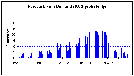
Simulation Case I
Probability = 100%
Units to be produced= 666

In the above simulation, we
see that if the firm produces 666 units, it will have a 100% probability of
selling them. To increase the profits, and take a calculated risk, the firm
decides to raise the number of units, and check the probability again, and this
is done in the following case.
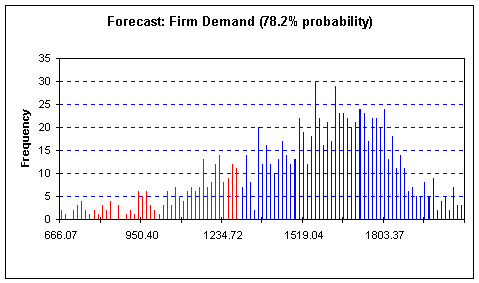
Simulation Case II
Probability= 78.2%
Units to be produced = 1300
When the output is raised to
1300 units, probability of achieving Firm Demand is 78.2%. Based on the information attained, it would
be advisable to go ahead with producing 1300 units.

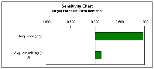
Sensitivity Chart
The software gives us the ability to view a sensitivity chart, which clearly shows that Average price is a major determinant in the Firm Demand, as 97% of the Firm Demand is dependent on it. The Average advertising comparatively plays an insignificant role.
