I. Objective
The objective of this project is to forecast demand (FD) for the company’s product, based on historical data.
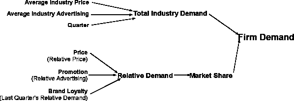
FD will be arrived at by examining two types of variables. One type will predict total industry demand (TID) and the other type will predict market share or relative demand (RD). Hence, FD=TID*MS, where MS=RD/N, where N is the number of companies in the industry.
Average price, average advertising, and time will be used to predict TID. Relative price, relative advertising, and last quarter’s relative demand will be used to predict RD.
Graphic Model

II. Description of Variables
TID variables
 |
 |
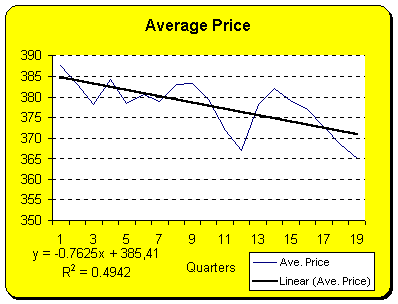 |
The three line graphs show that there are
trends in the variables over time. The upward trend in TID and the downward trend in Ave.
Price are much stronger then the upward trend in Ave. Adv. Only about 27% of the data can
be explained by the linear trendline. The two scatter plots below show that there is a strong correlation between TID and both Ave. Price and Ave. Adver. |
 |
 |
The correlation matrix gives important data on how the variables are related to one another:
| Quarter | Avg_Price | Avg_Adv | TID | |
| Quarter | 1.000 | |||
| Avg_Price | -0.703 | 1.000 | ||
| Avg_Adv | 0.522 | -0.749 | 1.000 | |
| TID | 0.695 | -0.889 | 0.882 | 1.000 |
The correlation matrix shows that TID is correlated with all of the variables. Unfortunately, some of the independent variables are highly correlated to each other, casting a doubt on their being independent.
A regression analysis of the three variables paints a telling picture. See the table below.
| Regression Analysis for TID using Quarter, Average Price and Average Advertising as independent variables | ||||||||
| Regression Statistics | ||||||||
| Multiple R | 0.9523 | |||||||
| R Square | 0.9069 | Taking a quick look at the table, it is obvious, that including Quarter in the analysis will probably result in a Type I error, since the P-value for Quarter is almost 22%. It is best not to include it. | ||||||
| Adj. R Squ. | 0.8883 | |||||||
| Regression Coefficients | ||||||||
| Coefficients | Stand. Err. | t Stat | P-value | |||||
| Intercept | 130249.28 | 50620.07 | 2.57 | 0.021 | ||||
| Quarter | 123.23 | 102.99 | 1.28 | 0.219 | ||||
| Avg. Price | -358.61 | 122.18 | -2.94 | 0.010 | ||||
| Avg. Adv. | 0.26 | 0.06 | 4.16 | 0.001 | ||||
By excluding the Quarter variable, the data becomes valid for constructing an equation for TID. See table below.
| Regression Analysis for TID using Average Price and Average Advertising as independent variables | ||||||||
| Regression Statistics | ||||||||
| Multiple R | 0.9470 | |||||||
| R Square | 0.8967 | After excluding the Quarter variable, the other variables P-values increased. Now all P-values are at an acceptable level. | ||||||
| Adj. R Squ. | 0.8838 | |||||||
| Regression Coefficients | ||||||||
| Coefficients | Stand. Err. | t Stat | P-value | |||||
| Intercept | 164336.17 | 43962.47 | 3.74 | 0.002 | ||||
| Avg. Price | -445.16 | 103.94 | -4.28 | 0.001 | ||||
| Avg. Adv. | 0.26 | 0.06 | 4.07 | 0.001 | ||||
Based on the table above, the following equation can be created:
TID=164336.17-445.16*Avg. Price+0.26*Avg. Adv.
This equation explains roughly 90% of all TID values based on Avg. Price and Avg. Adv.
RD variables
Relative demand, which is the firm demand divided by the industry average demand, will be predicted based on the following variables:
 |
 |
|
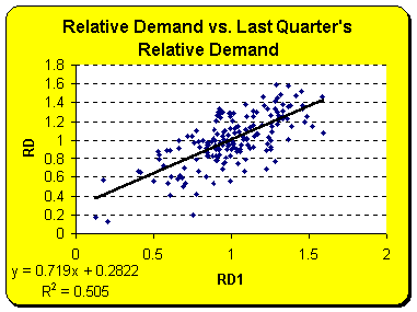 |
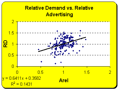
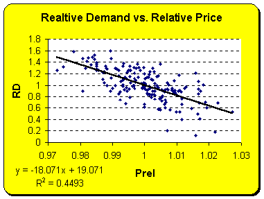
The scatter plots show that
two independent variables do correlate to the dependent variable, which is
relative demand. Relative advertising, however, does not correlate to
relative demand very much.
|
|
A correlation matrix is needed to get a better understanding of the relationship between all of the variables.
| RD | Prel | Arel | RD1 | |
| RD | 1.000 | |||
| Prel | -0.495 | 1.000 | ||
| Arel | 0.382 | 0.417 | 1.000 | |
| RD1 | 0.833 | -0.248 | 0.170 | 1.000 |
The correlation matrix confirms, that Arel is not very much correlated to RD, in fact it is more correlated to Prel. It can also bee seen, that the independent variables are not highly correlated to each other.
A regression analysis reveals how well RD can be predicted using the independent variables:
| Regression Analysis for RD, Using Prel, Arel, and RD1 as Independent Variables | ||||||
| Regression Statistics | It turns out from the regression analysis, that all independent variables are indeed independent, and the coefficients are able to explain roughly 95% of the values of Relative Demand | |||||
| Multiple R | 0.9785 | |||||
| R Square | 0.9575 | |||||
| Adj. R Squ. | 0.9568 | |||||
| Observations | 179 | |||||
| Regression Coefficients | ||||||
| Coefficients | Stand. Err. | t Stat | P-value | |||
| Intercept | 16.1300 | 0.4445 | 36.2862 | 0.0000 | ||
| Prel | -16.4445 | 0.4441 | -37.0255 | 0.0000 | ||
| Arel | 0.7796 | 0.0269 | 28.9347 | 0.0000 | ||
| RD1 | 0.5334 | 0.0164 | 32.4615 | 0.0000 | ||
Based on the table above, the following equation can be created:
RD=16.1300-16.4445*Prel+0.7796*Arel+0.5334*RD1
This equation explains roughly 95% of all RD values based on Prel, Arel and RD1.
III. Mathematical Modeling
Total industry demand can be computed by help of the equation:
TID=164336.17-445.16*Avg. Price+0.26*Avg. Adv.
Relative demand can be computed with the following equation:
RD=16.1300-16.4445*Prel+0.7796*Arel+0.5334*RD1
Relative demand can be used to compute market share using the equation:
MS=RD/n (number of firms: n=10)
Firm Demand can be computed with the help of TID and MS and the following equation:
FD=TID*MS
The final equation for FD is the following:
FD=(164336.17-445.16*Avg. Price+0.26*Avg. Adv)*(16.1300-16.4445*Prel+0.7796*Arel+0.5334*RD1)/10
| Inputs | Outputs | |||
| Industry Estimates | Total industry demand: | 37130.17 | ||
| Avg. Price (in $): | 350 | |||
| Avg. Advertising (in $): | 110000 | Relative Demand: | 0.595567 | |
| RD1: | 1 | |||
| Market Share: | 5.96% | |||
| Your Decisions | ||||
| Price (in $): | 345 | Forecasted Demand: | 2211.35 | |
| Advertising (in $): | 20000 |
Click here for a working spreadsheet model of firm demand.